Projects, Lessons Learned

BETTER FORECASTING OF PROJECT TIME AND COST OUTCOMES

A key role of the project controls practitioner is to help ensure that the forecast time and cost outcomes of a project when it is funded are as close as possible to the actual final outcomes. This poster presentation examines the track record across many sectors, assesses reasons for failure to succeed and explores ways in which forecasting can be improved.

THE PROBLEM – TOO MANY PROJECTS EXCEED BUDGETS & FINISH DATES

In fact the percentage by which projects exceed their original budgets can be high, especially for large and complex projects.

Affects all types of Projects and Sectors

An intriguing aspect of the problem is that it can be found right across the spectrum of sectors and types of industries. Examples of major overruns in a wide range of industry sectors are given below.

Defence

Australian Air Warfare Destroyer Program[1]

The Hobart class is a ship class of three air warfare destroyers (AWDs) being built for the Royal Australian Navy (RAN). Planning began in 2000. Although the designation “Air Warfare Destroyer” is used to describe ships dedicated to the defence of a naval force (plus assets ashore) from aircraft and missile attack, the planned Australian destroyers are also expected to operate in anti-surface, anti-submarine, and naval gunfire support roles.

Three ships were ordered in October 2007, at an announced cost of A$ 7.9bn. They are being assembled at ASC’s facility in Osborne, South Australia, from 31 pre-fabricated modules. ASC, NQEA Australia, and the Forgacs Group were selected in May 2009 to build the blocks, but within two months, NQEA was replaced by BAE Systems Australia. Construction errors and growing delays led the AWD Alliance to redistribute the construction workload in 2011, with some modules to be built by Navantia, the Spanish designer of the AWD.

Increasing slippage has pushed the original planned 2014-2016 commissioning dates out by at least three years, with lead ship Hobart to be handed over by June 2017, Brisbane in September 2018, and Sydney by March 2020. Originally, the Hobart-class destroyers were to be operational between December 2014 and June 2017. By March 2014, the project was running A$302 million over budget. By May 2015, this had increased to A$800 million, with a predicted minimum cost overrun by project end of A$1.2 billion. But according to a defence sector specialist, the likely total project overrun will be A$1.8 to A$2.3bn[2], say A$2.1bn.
The cost overrun to complete will be 2.1/7.9 = 27%; the time overrun will be 33 mths/116 mths = 28%.

A March 2014 report by the Australian National Audit Office (ANAO) heavily criticised the DMO and the AWD Alliance for underestimating the risks in redesigning the ships for Australian operations, and building them in shipyards with no recent warship construction experience. The ANAO report also criticised designer Navantia and the shipyards involved in block construction over poor drawings, repeated errors, and bad building practices. As a result of further delays and growing costs, the Hobart-class destroyer project was added to the government’s “Projects of Concern” list in June 2014. Follow-up government reports identified unrealistic time and cost estimates as additional factors. The overarching alliance concept has been repeatedly denounced, with no effective management structure or entity in charge, (allowing for repeated blame-passing between the individual alliance partners, Navantia, and the subcontracted shipyards), and the DMO locked in a contradictory role (simultaneously acting as supplier, build partner, and customer).

The weapons systems for the AWD vessels have been sitting in a warehouse for a decade and could be obsolete before they are used.[3] The Australian Strategic Policy Institute (ASPI), a government-funded think tank, says up to $5 billion has been earmarked for AWD upgrades before the other two ships have even started sea trials. That is about half the project’s entire budget.

Military technology expert James Mugg wrote in an ASPI report that it could be smarter to give up on the existing build, or at least upgrade them before they hit the water. “For $5 bn, the Royal Australian Navy could buy two larger, more capable (US) Arleigh Burke-class destroyers with the latest Aegis configuration … it would save money and possibly even receive the vessels before the upgrades to the AWDs are expected to be completed,” he wrote.

Insight Economics director Jon Stanford says it might be sensible to “cut our losses” and buy the US ships. “That would just look absolutely awful. But (the project) has just been messed up from the word go,” he told The Advertiser. “It should never have gone to Adelaide in the first place. Williamstown (Victoria) was just finishing the ANZACS. It had a superbly trained workforce; they had built ships on time and on budget.”

Joint Strike Fighter (JSF)[4]

The Joint Strike Fighter jet is Australia’s largest ever weapons purchase, but it’s four years late so far and well over budget. Australia’s jets were originally estimated at US$40 million each (when Australia bought into the program in 2002), which the government says has now escalated to US$90 million. But at this stage Australia is spending a total of almost AU$18 billion on its Joint Strike Fighter program, that’s more than $200 million per plane, excluding operating costs. Full life cycle costs are likely to exceed A$45 billion.
Despite it being the most expensive military item we’ve bought so far, it never went to tender.

The planes were due to start arriving in 2012, but it is unlikely any will arrive until at least 2020. Currently there are very serious problems relating to:

Overheating (above 32°C the weapons bay doors must be opened);
Software (25 million lines of code, being bug-fixed from 2013 to 2020)
Simulation (no verified simulation capability yet achieved, preventing performance capability testing)
Weight of JSF helmet (produces certain neck damage in an ejection, possibility of death)

Earlier in 2016, Canada pulled out of buying 65 JSFs. Australia has committed to buy 72. Watch this space…

Information Technology

Queensland Health Payroll System[5]

In 2002 the then Queensland Government established the “Shared Services Initiative” (SS Initiative, or the Initiative), the purpose of which was to amalgamate and rationalise government services such as accounting, human resource management and payroll across a number of departments and agencies. The Initiative was based on the Shared Services Model, an organisational approach which had been embraced by large corporations in the United States of America in the 1980s and had apparently been applied to the public sector with some success. But in Queensland it proved more difficult and costly to implement than the theory which underlay the Initiative suggested.

The SS Initiative formally commenced on 1 July 2003 with the establishment of four Shared Services providers and CorpTech which was a technology centre located within Queensland Treasury and was to become the technology service provider for the whole-of-government. In August 2005 the Shared Services Solutions Program (SSS Program) was established and required CorpTech to design and build a whole-of-government human resources and finance solution with a capital budget of $125m. Between then and November 2005, CorpTech undertook the evaluation of products and programs best suited to deliver human resource and payroll services for the SS Initiative. Relevantly for the functions of payroll and rostering, the products chosen were SAP ECC 5 and Workbrain, to be implemented by IBM Australia Ltd (IBM), the Workbrain licencee.

As part of the SS Initiative, in March of 2006 Queensland health (QH) had transferred responsibility for the maintenance of human resource software and hardware to CorpTech. At this time the provision of a new computerised payroll system for its employees was thought to be urgent because the existing system, known as LATTICE, was nearing the end of its useful life. The supplier and licensor of the system had declared it would not service or update it after 30 June 2008 and a new enterprise bargain under negotiation between QH and its employees would add to the complexities of payroll calculation which LATTICE could not accommodate.

CorpTech made little progress. It engaged a large number of contractors on a “time and materials” basis to assist with its design and implementation of the solutions. These engagements were costly and not always efficient. Finance solutions were successfully deployed to about 12 agencies, but Payroll proved more difficult. Only the Department of Housing was brought online, without complete success.

In 2006/7, the SS Initiative was the subject of a review, which resulted in a quest to devolve responsibility for the design and implementation of the SS Initiative to a single contractor. A detailed Invitation to Offer was issued to four shortlisted companies and, from the three that responded IBM Australia was contracted in December 2007 to provide Shared Services to nominated departments. The replacement of QH Payroll was to be the first system delivered, by 31 July 2008.

The change of strategy was unsuccessful. By October 2008 IBM had not achieved any of the contracted performance criteria; but it had been paid about $32m of the contract price of $98m; and it forecast that to complete what it had contracted to undertake would cost the State of Queensland $181m. Accordingly the Shared Services Solution across the whole-of-government was abandoned and IBM’s contract was reduced in scope to providing a new payroll system for QH.

QH was the largest single department of government with the most complex workforce arrangements. About 80,000 staff members were covered by 12 different industrial awards and were affected by six different industrial agreements. These together created more than 200 separate allowances and as many as 24,000 different combinations of pay. Of all departments it was the most difficult for which to design a payroll system.

On 14 March 2010 after ten aborted attempts to deliver the new payroll system, it “went live”. It was a catastrophic failure. The system did not perform adequately with terrible consequences for the employees of QH and equally serious financial consequences for the State. After many months of anguished activity during which employees of QH endured hardship and uncertainty, a functioning payroll system was developed, but it was very costly. It required about 1,000 employees to process data in order to deliver fortnightly pays. It was estimated that it would cost about $1.2b over the following eight years. The replacement of the QH payroll system must take a place in the front rank of failures in public administration in this country. It may be the worst.

The Chesterman Inquiry ^(ibid,5) listed a number of Lessons Learned, including the following:

There were two principal causes of the inadequacies which led to the increase in contract price, the serious contract and project management shortcomings, and the State’s decision to settle with IBM.
Those causes were: unwarranted urgency and a lack of diligence on the part of State officials. That lack of diligence manifested itself in the poor decisions which those officials made in scoping the Interim Solution; in their governance of the Project; and in failing to hold IBM to account to deliver a functional payroll system.
These problems are not ones which should be thought to be unique or unlikely to arise again. The particular circumstances of this failure may not recur, but the problems are systemic to government and to the natural commercial self-interest of vendors. They are commonly experienced in projects of this kind.
This Project has provided strong evidence that the State, try as it might, cannot outsource risk. The desire to outsource to the private sector requires the government actively and competently to manage projects and contractors, and apply the necessary skill and expertise to ensure the effective delivery of large projects. The State cannot be passive in its oversight of projects in which large amounts of taxpayers’ money are at risk or the welfare of State employees may be affected.

Three Recommendations were made by the enquiry, including the following:

The Queensland Government apply an appropriate structure to oversee large ICT projects, to ensure:
- that the relevant individuals have skills in project management and
- the power to make inquiries and to report to senior public officials.

Merging of Customs and Immigration IT Systems

An IT project for the Australian Government is in trouble. IBM has missed a 31Oct16 deadline to merge the Customs IT system (run by IBM) and the Immigration IT system being run by CSC. In mid-October, the Deputy Secretary of the Department of Immigration and Border Protection (DIBP) told a Senate committee the revised deadline was early December. CSC’s contract has been extended to January 2017. Watch this space…

Infrastructure

Victorian Desalination Project[6]

The Victorian Desalination Plant (also referred to as the Victorian Desalination Project or Wonthaggi desalination plant) is a 150 gigalitres per year water desalination plant in Dalyston, on the Bass Coast in southern Victoria, Australia, completed in December 2012. As a rainfall-independent source of water it complements Victoria’s existing drainage basins, being a useful resource in times of drought. The plant is a controversial part of Victoria’s water system, with ongoing costs of $608 million per year despite virtually no utilisation since completion. The first delivery of 50 gigalitres of water is to be supplied in 2016.

Background

The total average inflow into Melbourne dams from 1913 to 1996 was 615 gigalitres per year, whilst average inflow 1997–2009, during the most severe drought ever recorded in Victoria, was 376 gigalitres per year. Rapid population growth also put pressure on reserves. Reserves in the state’s water storage dams decreased from 1998 to 2007 to around a third of maximum capacity. Severe water restrictions were introduced and Melburnians began to worry about running out of water.

By June 2007, the Victorian Government released its water management strategy marketed as Our Water Our Future. As part of the plan, the government announced its intention to develop a seawater reverse osmosis desalination plant to “augment Melbourne’s water supply, as well as other regional supply systems.”

An Environmental Impact Statement Report was issued in August 2008 and eight tenderers submitted offers, from which two consortia were shortlisted. The AquaSure consortium of Degremont, Thiess and Macquarie Capital was selected on 30Jun09, with a commitment to deliver First Water in late 2011, about 30 months from the official selection date.

The site selected was on a flood plain next to a wind farm in the old Powlett River coal fields of Wonthaggi, on the coast. Seawater is drawn from Bass Strait, about 1.2km offshore. The plant is about 500m from the coast. About half the intake seawater is returned into a separate offshore discharge location as doubly concentrated brine.

The plant is estimated to require 90 MW of electricity to operate. Additional energy is required to pump the desalinated water from Wonthaggi to Cardinia Reservoir in Melbourne. A windfarm was built elsewhere to compensate for the power required.

Cost

The capital cost for the project was initially estimated to be $2.9 billion in the initial feasibility study; this was later revised to $3.1 billion and then to $3.5 billion. After the winning bidder was announced it was revised to $4 billion. The project is a Public Private Partnership, with the AquaSure consortium responsible for building, owning and operating the plant.

There are two revenue streams for the plant:

An operating cost for production of water; and
An availability fee of about $1.8m per day for the standing and financing costs of the plant, effectively an insurance premium charge for being able to provide water when needed.

The minimum fee payable for a total of 27 years after completion, even if no water is required, totals between $18 and $19 billion. The average water bills for residents living in Melbourne were estimated to rise by around 64% over the period 2008-2013. Water price plans released by the Essential Services Commission illustrated that metropolitan water providers would charge between 87 per cent and 96 per cent more for water.

Schedule

The contract for the project was signed in an atmosphere of deep concern about the risk of Melbourne running out of water. Liquidated damages were set for penalties of around $400m for late delivery of the project. The plant was commissioned about 12 months after the original due date, an overrun of 12/30=40%. Delays were caused by a range of factors including:

Industrial unrest
Flooding of the site
High winds hampering steel and equipment erection progress
Significantly underestimated complexity and duration of pumping facilities civil works.

Project Outcomes

The project was handed over for operation in December 2012. Arising from the delays and other problems, the main parties in the AquaSure Consortium – the designers Degremont (part of French conglomerate GDF Suez) and the constructors Thiess (part of then Leighton Holdings, now CIMIC) were expected to lose more than $800m.[7] Thiess initiated legal action against AquaSure.[8] The commercial outcomes have not been made public, but the Victorian Desalination Plant was a significant part of Leighton Holding’s financial problems in that period, along with the Queensland tollway project, Airport Link.

Mining

There were many projects that overran original time and cost forecasts in the boom decade between 2004 and 2014. Many overran due to shortages of skilled resources to develop and deliver the projects. In the latter stages of the boom, projects were cancelled due to the realisation of the business risk that revenue would not meet the required project RoI due to falling commodity prices. Two related example BHP projects are described below which were ultimately affected by the falling price of nickel.

BHP Ravensthorpe & Yabulu Projects (2004-2008)[9]

Introduction

BHP was determined to expand its nickel production, following acquisition of Western Mining Corporation’s (WMC’s) nickel business, as part of its goal of only being in Tier 1 assets. Metallurgically, the simplest nickel ores to process, magmatic sulphides, are in increasingly short supply and mostly the more difficult lateritic nickel ores are available, which required high pressures, acidity and temperatures to extract the nickel concentrates (Robinson, 2012) . A limited life lateritic ore body was available near Ravensthorpe in SW WA which required the above still novel processing. BHP Billiton had inherited a 30 year old nickel refinery from Billiton in Townsville which it decided to upgrade substantially to process concentrate from Ravensthorpe.
BHP engaged the company which had bought its engineering organisation to be the EPCM contractor for both linked projects.

When announced in March 2004, on a rising market, the combined Ravensthorpe and Yabulu projects were estimated to cost US$1.4bn and deliver an extra 44,500 tonne/y of nickel and 1,400 tonne/y of cobalt from the Yabulu Refinery giving totals of 76,000 t/y of nickel and 3,500 t/y of cobalt. The first shipment of concentrates from Ravensthorpe to Yabulu was forecast to occur in Q2, 2007 and the first Yabulu metal production from those concentrates in Q3 2007. The actual performance of the two projects was rather different.

Ravensthorpe nickel Mine & Concentrator

The process chosen was still not fully proven at production scale and required High Pressure (Sulphuric) Acid Leaching (HPAL). The Ravensthorpe Nickel Concentrator site during construction is shown in Figure 3 below.

Design, procurement and construction of the project required several re-baselinings and there was a lot of interference by BHP in process finalisation and equipment definition and selection, along with approval delays. The project had to go back to the BHP board multiple times for additional funding and completion was delayed substantially. While the EPCM contractor was far from blameless, they submitted claims to BHP for hundreds of thousands of extra manhours based on delay, disruption and scope changes.

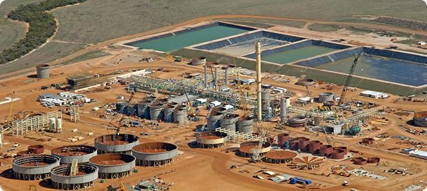Ravensthorpe Nickel Concentrator during construction

Source: http://www.ertech.com.au/experience/resources-experience/ravensthorpe-nickel-project/

The mine and processing facility were completed in late 2007 at a cost of US$2.2bn and started up with difficulties. They were officially opened in 2008, with production expected to reach 50,000 t/y of included nickel.

The Ravensthorpe rampup coincided with the Global Financial Crisis and a severe decline in the price of nickel. The price dropped to around US$10,000/tonne, less than 1/5^th of the peak price of ~US$54,000/tonne in 2007:

In January 2009 (around the time of the minimum price for nickel), BHP Billiton shut down the Ravensthorpe mine and plant, after less than a year of operation, and put them on the market.

Yabulu Nickel Refinery Townsville

A similar story unfolded with the Yabulu Nickel Refinery near Townsville. The 30 year old Greenvale nickel refinery was more than doubled in size in a brownfields expansion to handle the nickel concentrates to be produced from Ravensthorpe. The project had a number of interfaces with the existing operating refinery, which greatly complicated the construction, as did the need for extensive refurbishment of the original refinery. Approval delays and design changes from the owner / operators, along with chronic delays to provision of certified vendor data required for model finalisation and issuance of AFC drawings resulted in cumulative disruption of the project. Again claims were submitted to BHP for hundreds of thousands of extra manhours.

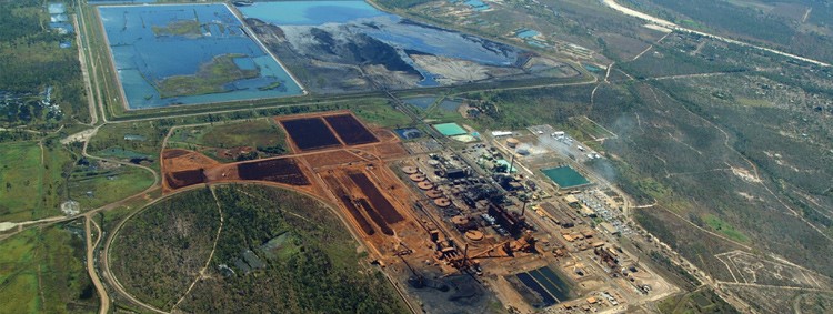Yabulu Nickel Refinery

Source: http://trility.com.au/projects/qni-yabulu-reuse-plant-reference-site/

Yabulu received its first mixed hydrate matte from Ravensthorpe in early 2008. After less than a year of production, the matte-processing stream in the refinery was shut down in January 2009, concurrent with the shutdown of Ravensthorpe.

Final Project Outcomes

In July 2009 BHP Billiton sold the Yabulu Nickel Refinery to Clive Palmer for an undisclosed amount and wrote down the carried value of the refinery by US$500m and a further US$175m in unrecoverable tax losses. The price of nickel, which had peaked at around US$55,000/tonne in 2007, had fallen to ~US$10,000 in mid-2009.

At the end of 2009, BHP Billiton sold the Ravensthorpe mine and plant to Canadian company First Quantum Minerals (FQM) for US$340m. After 18 months of modifications and recommissioning, the mine and concentrator re-opened, producing nearly 33,000 tonnes of included nickel in 2012, its first year of operation.

The write-downs by BHP Billiton for Ravensthorpe and Yabulu totalled US$3.6bn.

The acquiring companies owning and operating the mine and the refinery at first made a success of them in market conditions where product could be sold at around twice the price that prevailed when BHP shut down the ventures. They were able to purchase major facilities at highly discounted prices. However, since then nickel prices have fallen again, dipping as low as when BHP decided to close the projects. This caused the closure of Clive Palmer’s Townsville Nickel Refinery in late 2015. Ravensthorpe came close to closing earlier in 2016 as attempts were made to sell it. But the nickel price has since risen from ~ US$10,300 to ~US$11,700.

As of November 2016, FQM was still operating Ravensthorpe. Whether it can keep operating depends ultimately on future movements in the nickel metal price.

Oil & Gas

Woodside Pluto Project (2007-2012)[10]

Introduction

Woodside Petroleum Ltd was proud of its relatively quick development of the Pluto project from initial field discovery in 2005 to FID and construction of the facilities. Compared with other greenfields LNG projects, it was initially very speedy. The scope of the project provided for 5 subsea wells from the 4.5 TCF Pluto and Xena gas fields in 800m of water 180km offshore from the Burrup Peninsula to supply a 4.3 MTPA single train LNG plant. This was Woodside’s first 100% owned LNG project.

In November 2006, at an Industry Briefing on the project, Woodside accurately forecast Financial Investment Decision to occur in July 2007, but optimistically forecast First Cargo could occur in October 2010, a project duration of only 39 months. The project took much longer.

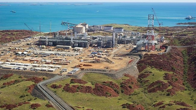Pluto LNG Plant nearing completion

Source: http://www.perthnow.com.au/business/woodsides-pluto-project-finally-ready-to-roll/story-e6frg2s3-1226307656878

Pre-Financial Investment Decision (FID) choices and consequences

The front-end planning of Pluto by Woodside was performed in a short time (FEED started September 2006, FID July 2007). It is understood that Woodside management made a conscious decision to proceed to FID and execution phase with minimal delay, in their desire to bring the gas to market as early as possible.

Woodside and their Onshore EPCM Joint Venture contractor for Pluto, Foster Wheeler (60%) Worley Parsons (40%) (FWWP) were in an integrated team relationship for NW Shelf LNG Train V completion and startup (starting up in 2008), which were happening in parallel with the early stages of Pluto. Woodside management established a conventional EPCM contract with the FWWP JV for Pluto.

The complexity and scale of the challenge of assembling skilled and experienced engineering resources to design and manage the procurement and construction of the onshore facilities in a stretched project environment in Australia and elsewhere, in offices servicing other parts of the overheated Australian market resulted in material problems and delays to the onshore scope as described below.

Engineering, Logistics & Quality Problems

These problems of complexity and over-stretched resources showed up initially in late engineering and procurement. As is now normal for such complex plants, the plant was modular in design, to maximise fabrication and pre-assembly in more efficient and lower unit cost module yards in SE Asia and minimise expensive site construction labour costs. However, this imposes tighter deadlines on engineering and procurement to ensure equipment is designed into modules and the equipment and materials are specified and procured in time to be installed in the module yards for scheduled shipment to site.

The materials had to be available in time to achieve the required installation schedules in the modules to comply with the fixed shipping schedules of the large module carrier vessels which shuttled between the yards and the Burrup Peninsula to deliver the modules. Due to late engineering and procurement, FWWP / Woodside were faced with a difficult choice of shipping modules incomplete, to be completed on site, or delaying the module shipments until the materials were available, thus incurring delay costs from the shipping company and additional charges from the module yard owners, who had following work from other clients and restricted space for storage. As a consequence, carry-over work and completion of work out-of-sequence in the modules on site became a major issue.

This situation was made significantly worse by module quality problems requiring substantial rework onsite. A further exacerbating factor was the increased difficulty of installation work inside modules compared with non-modularised plant. It has been estimated that 100 manhours of work in a module yard, where the modules are spread out for assembly access, requires 200 manhours of work on site where the modules have already been assembled. This is quite apart from the substantially higher cost of labour on site.

The increased site work was quarantined from the main project team. The integrated project team option used on NWS Train V was implemented and a task force run in parallel to manage the out-of-sequence, carryover and rework, so the main project management team was not diverted from completing the project.

Reduction of Team Motivation by Project Plan

The Pluto Project used a countdown calendar to “Ready For Start Up” (RFSU). The publicly announced target onshore RFSU of 27 Aug 2010 was unable to be met because of the above engineering, logistics and quality problems and industrial disputes that followed late in 2010 and 2011. This meant that the countdown calendar lost its utility as a motivator for the project team and the schedule behind it was at risk of ceasing to be a useful guide for the project team until it was re-baselined.

Industrial Relations Consequences of Acceleration of Work Attempts

The previously mentioned out-of sequence, carryover and rework requirements put great pressure on completion of the onshore scope because the authorised and prepared construction area was quite restricted and the remote location imposed strong accommodation constraints. To deal with the added workload and the need to increase manning to minimise slippage, in late November 2009, Woodside changed the accommodation rules from one room for exclusive use of each worker to “motel-style” accommodation, where worker’s personal belongings were stored, but when each worker went on R&R, another incoming worker would take their place. This freed up 25% of the accommodation, but also caused a major industrial dispute in January 2010 and significant delay to the project. Industrial action may have added 6 months to the Pluto construction duration.

Offshore Costs Blowout

Offshore costs blew out significantly, driven more by labour rate increases and work practices than prolongation costs. The sharp increase in rates followed the implementation of the Fair Work Act 2009. The Offshore Hydrocarbons Construction Rate increased 184% in the years 2005-2011, increasing from 481% to 663% of Average Weekly Earnings for Australia.

Final Project Outcome

The actual First Cargo departed on 12 May 2012, 58 months after FID (July 2007), at least 12 months later than realistically expected. The overrun compared with the originally announced 39 months was 58/39=49%.
The original estimate for the cost of the Pluto Project was $12bn, which became around $15bn, an increase of about 25%. Pluto has been operating successfully since, albeit since 2014 in a much lower LNG Price environment.

Comparison with Chevron Gorgon Project

Even after this delay, the Pluto development duration from field discovery to first product of around 7 years was still fast compared with most other Greenfield LNG projects. For example the first Gorgon field gas was discovered 33 years ago, with first LNG expected at FID in 2014, but actually achieved in March 2016, 78 months after FID. Its initial budget was announced as US$37bn at FID in September 2009, but grew to more than US$55bn, a cost overrun of nearly 50%.

MANY REASONS FOR OVERRUNS

As can be seen from the foregoing examples of projects that have exceeded time and cost forecasts, there are many reasons. However, certain common patterns of causes can be found.

Deficiencies in organisation(s) developing and delivering the project

Systemic deficiencies in the organisations planning and executing the projects are probably the most common causes of overruns. If the organisation is not capable of developing and delivering the project through inadequacies in structures, leadership personnel, procedures and practices, the initial planning, estimating and design of the project are likely to be inadequate and late; while problems that arise will be exacerbated.

Predetermined total time and cost targets[11]

Many projects are planned to fit in with predetermined dates of completion, rather than to provide durations required to complete the scope. This situation is often exacerbated by slippage of the timing of project commencement without corresponding delay to the project completion date. Whether due to fear of loss of face for company management or due to politically imposed deadlines, such schedule compression reduces the probability of timely completion, although it is unlikely to be apparent from viewing the project plan.

Inadequate front end design, planning and estimating of the project[12]

Independent Project Analysis, Inc. (IPA), reported (Young, 2009) that 74% of completed Large and Technically Complex Projects assessed by IPA in Australia had been failures, mainly due to deficiencies or omissions during planning of the projects before they were approved for execution.

In late 2012, PricewaterhouseCoopers (PwC) reported that most projects failed to deliver at least some of their benefits and be completed within the planned time and cost limits and that over 90% of these failures were due to management failings rather than technical problems.

2.2 Single value estimates of time and cost tend to be optimistic¹¹

Project planning tools such as Primavera P6 or Microsoft Project require the user to input single durations for each task defined as part of the project plan. Connecting up all the single-duration tasks with appropriate logic determines the end date through application of the rules of the critical path method to find the longest path through the project schedule, along with all the early and late dates for the rest of the tasks in the schedule. This is why such software is described as deterministic – there is only one date able to be determined for the project completion once the start date is defined. When there is pressure to produce an expected date that may have been pre-announced it is hard to avoid incorporating optimism in the durations.

In reality the duration of a task is rarely able to be known exactly. In most cases, it is more like being asked how long it takes to travel from home to work each day. Because it is a regularly repeated activity, most people are likely to answer in a way similar to the following:
“If it is a fine day when most people are away on holidays, it only takes me 20 minutes. In winter, when the weather is bad and everyone is trying to get to work, it may take 50 minutes. If there is an accident or the road is being repaired, it can take 75 minutes. Most of the time it takes about 30 minutes.”

Project plans contain hundreds or even thousands of activities like this. But deterministic project planning only allows one duration value for each task. The project planners cannot represent the inherent uncertainty of each task in their single duration values. Consequently, when the pressures of producing the desired end date are factored in, the likelihood of the schedule being inherently optimistic is high.
If the project cost estimate is aligned with the schedule durations, it also is likely to be optimistic.

Monte Carlo Method range analysis – a solution to single duration values¹¹

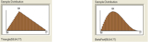
Task 3-point probability duration distributions

By replacing single durations with duration probability distributions we can represent the inherent uncertainty of activities in the project schedule. For example, the following two probability distributions represent a task of between 58 Minimum and 77 days Maximum duration, with a Most Likely (highest probability) duration of 64 days:

The two probability distributions – Triangular and Beta Pert – represent different ways of expressing how likely the task duration is to be around the Most Likely value (more likely using Beta Pert) or alternatively, spread more toward the extremities (Triangular). Other shapes can be used, but the value of replacing the single durations with probability distributions is realised by applying software using the Monte Carlo Method (MCM), a mathematical technique for simulating running the project hundreds or even thousands of times, randomly sampling the duration of each uncertain duration task in the schedule for each critical path calculation of the project schedule. The early and late dates and float for each task are stored for each critical path calculation or “iteration” and the software samples the duration values so that over the pre-determined number of iterations of the MCM simulation, from say 500 to 10,000, the sampling frequency for each task matches its predefined probability distribution. The object is to simulate as many possible combinations of task durations to produce the full range of project time outcomes as could realistically be expected to occur. Through this method, probability distributions are generated for the dates of all uncertain duration activities in the project schedule, including the end date. An example output is shown below, produced from Oracle’s Primavera Risk Analysis™ (“PRA”, formerly known as Pertmaster Risk Expert):

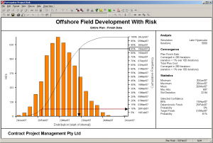The histogram plots the date outcomes for the completion milestone of the project of all the 5,000 iterations in the simulation, from earliest (left edge of the horizontal date axis) to the latest (right edge). The height of each orange bar represents the number of iterations (“Hits”) out of the 5,000 comprising the simulation, for which the PRA critical path software calculated the finish date between the left and right edges of the bar, shown on the left hand vertical axis. The cumulative curve overlaid on the histogram adds each successive bar’s iterations to the sum of the bars preceding it, such that the right hand vertical axis represents the cumulative number of iterations out of the total. So a horizontal intercept from the cumulative curve represents the probability that the project will be completed on or before the date vertically below the intercept on the cumulative curve.

Through using Monte Carlo Range Analysis we can answer questions, based on substituting duration distributions for single values, such as “How likely is the project to be completed by the planned date?” Or “What is a likely date for completing the project?” (e.g., 50% probable or P50 date is 24Mar above).

If we also overlay the schedule with the project cost estimate, dividing the costs appropriately into fixed (time-independent) and variable (time-dependent) costs, which are ranged in an analogous way to the durations, similar cost histograms and cumulative probability curves are produced at the same time. So we can overcome the tendency for optimism inherent in using single durations for project planning by using MCM Range Analysis and careful assessments of duration ranges used as inputs.

Failure to account for overlapping of converging logic pathways¹¹

Merge Bias Effect Of Converging Parallel Logic

All but the simplest project plans consist of multiple logic pathways that necessarily converge through milestone logic nodes leading to project completion. The probability of completing a given logic node milestone by the planned date is the determined by the probabilities of each pathway to that convergent node. How those probabilities are related to each other can be illustrated by the following example. Two identical activities are to be performed in parallel using identical but separate resources. If the probability of each activity A & B being completed by the planned finish date is 20%, what is the probability of both being completed by that date?

As shown at right, the probability of both tasks A & B being completed by the planned finish date is the product of the probabilities of each path being finished by that date. This is analogous to the probability of throwing two dice and getting the same value on each.

It is known as the Merge Bias Effect (MBE) and explains why it is hard to complete complex projects on time, due to the convergence of many parallel logic strands.

So when a project is delayed in starting, one effect is to reduce the probability of each logic pathway being completed by the planned date. Due to the MBE, the reduction in probability with project delay is geometric not linear, due to the probability of timely completion being the product of all converging probabilities.

Inadequate allowance for risk events¹¹

Earlier we discussed the time required to get to work from home and referred to the occasional traffic accident or road repair or malfunctioning traffic lights. Each of these is a Risk Event that has a low probability of occurrence, but in a project with thousands of activities, some risk events are virtually certain of happening. It is therefore essential to take risk events into account in planning such projects, to increase the resilience of the project, not only to such “known unknowns” that are identified and managed in the project risk register, but also to the inevitable “unknown unknowns” that occur in almost all projects and for which projects require a buffer of time and cost contingency. Projects that are planned with no allowance for risk events have no protection against unplanned threats to the project objectives. This can be seen as naïve optimism.

MCM simulation of the project can be broadened to allow for risk events as well as range uncertainties. The significant risks, both threats and opportunities with cost and schedule impacts in the project risk register can be mapped into the MCM model of the project and their effects taken into account through the product of their probabilities and impacts. By assessing the cost and schedule impacts of the risk events as three-point distributions, the uncertainty of the risk events can be allowed for both in their probabilities of occurrence and their impacts if they do occur.

AACE INTERNATIONAL ADDRESSES PROJECT OVERRUNS

AACEI TCM FRAMEWORK

Total Cost Management (TCM) is defined as “the effective application of professional and technical expertise to plan and control resources, costs, profitability and risks systematically throughout the life cycle of any enterprise, program, facility, project, product, or service.” The Framework is a structured, annotated process map that explains how each practice area in the cost engineering field relates to all the others and to allied professions. A free digital version of the TCM Framework comes with membership of AACEI.[13]

RELEVANT AACEI RECOMMENDED PRACTICES

AACEI has a wide range of Recommended Practices (RPs) that provide in straightforward language, guidance in how to use best practice in various processes required of Cost Engineers and related professionals, including Project Planners, Estimators, Cost Controllers and Risk Analysts and Managers. Listed below are RPs applicable for assessing time and cost impact risk in projects and thus determining appropriate levels of contingencies, with some comments added by the author.

VARIOUS APPROACHES TO ASSESSING & OPTIMISING PROJECT RISK

While there is general agreement about the need to assess and quantify time and cost risk in projects, there are a wide range of methodologies recognised and used for doing this. Here are some of the main ones.

GENERAL PRINCIPLES

Title: CONTINGENCY ESTIMATING – GENERAL PRINCIPLES
AACEI Recommended Practice No. 40R-08.
Scope: Defines the expectations, requirements, and general principles of practice for estimating contingency, reserves and similar risk funds (as defined in RP 10S‐90) and time allowances for project cost and schedule as part of the overall risk management process. The RP provides a categorization framework and provides a foundation for, but does not define specific contingency estimating methods that are covered by other RPs.

Comment: This RP is the statement of principles for any effective methodology for estimating project contingency. It lists the general principles then describes them in more detail. It describes classes of methods used to estimate time and cost contingency that can meet 40R-08 requirements. These are: Expert Judgment, Predetermined Guidelines, Simulation Analysis, Range Estimating, Expected Value and Parametric Modeling. Most of these are covered by the following specific RPs, which can include hybrid combinations of these.

PARAMETRIC

Title: RISK ANALYSIS AND CONTINGENCY DETERMINATION USING PARAMETRIC ESTIMATING
AACEI Recommended Practice No. 42R-08
Scope: Defines general practices and considerations for risk analysis and estimating cost contingency using parametric methods, commonly associated with estimating cost based on design parameters (e.g., capacity, weight, etc.). In this case, the method is used to estimate contingency based on risk parameters (e.g. level of scope definition, process complexity, etc.).

Title: RISK ANALYSIS AND CONTINGENCY DETERMINATION USING PARAMETRIC ESTIMATING – EXAMPLE MODELS AS APPLIED FOR THE PROCESS INDUSTRIES
AACEI Recommended Practice No. 43R-08
Scope: This RP is addendum to the RP 42R-08. It provides three working (Microsoft Excel®) examples of established, empirically-based process industry models of the type covered by the base RP; two for cost and one for construction schedule. The example models are intended as educational and developmental resources; prior to their use for actual risk analysis and contingency estimating, users must study the reference source documentation and calibrate and validate the models against their own experience.

Comment: Parametric estimating methods are generally simple to use. The challenge is to collect the data based on previous relevant projects and to develop the parametric models applicable to your project. This is an approach that requires a good database of prior project experience and thorough model development. However, parametric methods are particularly useful for assessment of the effects of systemic risks.

EXPECTED VALUE

Title: RISK ANALYSIS AND CONTINGENCY DETERMINATION USING EXPECTED VALUE
AACEI Recommended Practice No. 44R-08
Scope: This RP applies specifically to using the expected value method for contingency estimating in the risk management “control” step (i.e., after the risk mitigation step), not in the earlier risk assessment step where it is used in a somewhat different manner for risk screening. This RP is limited to estimating cost contingency.

Title: INTEGRATED COST AND SCHEDULE RISK ANALYSIS AND CONTINGENCY DETERMINATION USING EXPECTED VALUE
AACEI Recommended Practice No. 65R-11
Scope: This RP is an extension of 44R‐08. Because integrated cost and schedule methods are generally recommended, this RP has been created.

Comment: Both of these methods make use of the equation:
Expected Value (EV) = Probability of Risk Occurring x Impact If It Occurs
The method when applied to schedule impacts has the advantage over Critical Path Methods of not requiring a high quality schedule. However, due to schedule dependencies, parallel paths and float, use of the EV method requires a good understanding of scheduling as well as risk analysis. The method allows assumptions of project team risk responses in making schedule/cost trade-offs and requires a contingent response plan to be defined. It also requires correlation to be defined between cost and schedule impacts, which can be positive or negative. The EV Cost RP can be combined with the parametric methods for systemic risks.

SCHEDULE RISK ANALYSIS (SRA)

Title: CPM SCHEDULE RISK MODELING AND ANALYSIS: SPECIAL CONSIDERATIONS
AACEI Recommended Practice No. 64R-11
Scope: This RP does not present a standalone methodology, but is an extension of other RPs that present CPM-based approaches to schedule risk analysis and contingency estimating. This RP discusses key procedural, analytical and interpretive considerations in preparation and application of a CPM model; considerations not covered in the broader methodological RPs.

Comment: This is a valuable RP that takes the reader through the important issues and characteristics required to perform realistic SRA. It includes most considerations that matter.

COST RISK ANALYSIS (CRA)

Title: RISK ANALYSIS AND CONTINGENCY DETERMINATION USING RANGE ESTIMATING
AACEI Recommended Practice No. 41R-08
Scope: This RP describes a methodology to determine the probability of a cost overrun (or profit underrun) for any level of estimate and determine the required contingency needed in the estimate to achieve any desired level of confidence. The process uses range estimating and Monte Carlo analysis techniques.
What is Range Estimating? Range estimating is a risk analysis technology that combines Monte Carlo sampling, a focus on the few critical items, and heuristics (rules of thumb) to rank critical risks and opportunities. This approach is used to establish the range of the total project estimate and to define how contingency should be allocated among the critical items. The main uncertainty in the project estimate is assumed to be concentrated in a few critical items (typically 20 or less), using the Pareto Principle. The RP warns that the process must be followed rigorously or the estimated contingency will be understated.

Comment: Range Estimating is not conventional CRA, which typically ranges the whole estimate (sometimes called Cost Range Analysis), applies correlation or risk factors and adds in uncertain risk events. Conventional CRA requires assumptions when expressing time delay uncertainties or risk events to convert them to time-dependent costs for Monte Carlo analysis.

INTEGRATED COST & SCHEDULE RISK ANALYSIS

Title: INTEGRATED COST & SCHEDULE RISK ANALYSIS USING MONTE CARLO SIMULATION OF A CPM MODEL
AACEI Recommended Practice No. 57R-09
Scope: This RP defines the integrated analysis of schedule and cost risk to estimate the appropriate level of cost and schedule contingency reserve on projects. The main contribution of this RP is to include the impact of schedule risk on cost risk and hence on the need for cost contingency reserves. Additional benefits include the prioritizing of the risks to cost, some of which are risks to schedule, so that risk mitigation may be conducted in a cost-effective way and probabilistic cash flow which shows cash flow at different levels of certainty.
The RP methods integrate the cost estimate with the project schedule by resource-loading and costing the schedule activities. The probability and impact of risks/uncertainties are specified and the risks/uncertainties are linked to the activities and costs that they affect. Using Monte Carlo techniques one can simulate both time and cost, permitting the impacts of schedule risk on cost risk to be calculated.

Comment: This RP was written by Dr David Hulett author of two important reference books on SRA and this process of Integrated Cost-Schedule Risk Analysis (ICSRA) – see “Books” section below. The RP recognises the direct influence of delays on time-dependent costs in a project and solves the problem of how time and cost uncertainties and impacts interact by analysing them together. The RP describes the required inputs, the tools, the process and the outputs. A sample case study is worked through, including risk mitigations and probabilistic branching to simulate risk treatments.

Serial SRA to CRA

In contrast to the process described in RP 57R-09, most practitioners and organisations around the world wanting to integrate cost and schedule risk analyses use a two-stage process that can be called Serial SRA to CRA (SRA2CRA) because it is easier than ICSRA. In it, a summary schedule representing the project is created and used to perform an SRA. The project contingency duration is selected and transferred into a separate CRA, converted into a schedule contingency cost allowance assuming an average cost per unit time. All other cost line items are ranged in the CRA. Risk events from the project risk register of applicable impact types are mapped into the analyses. The method separates the schedule driven costs from their drivers, preventing the ranking of all sources of cost uncertainties in the one listing, hindering effective risk optimisation.

NASA JCL

A version of ICSRA has been successfully adopted by NASA from 2009, called joint Confidence Limits (JCL). JCL requires project funding requests to be based on P70s for both schedule and cost. This has been very successful, as an audit report showed in 2015[14]. 10 projects completed since the introduction of JCL were completed on average under their forecast costs, compared with the decade before JCL, in which 85% of NASA projects exceeded their budgets by an average of 53%. The audit also reported improved communication and project management practices resulted from the use of JCL.

AACEI TO COMPARE APPROACHES TO ASSESSING CONTINGENCIES

Project Risk Quantification Methodologies 2017 Annual Conference Track

At their 2017 Annual Meeting, 11-14Jun17 in Orlando Florida, AACEI is running a special conference track: “Project Cost and Schedule Risk Quantification Methods: Alternative Methods” to explore the different methods used for estimating time and cost contingency. Abstracts have been accepted from many parts of the world representing a range of industry sectors. A closing panel discussion will use a compiled table of methods as a focal point of discussion.
The goal is to update RP 40R-08 “Contingency Estimating – General Principles” with a comparative table of methods including their pros and cons.

FURTHER INFORMATION

The interested reader is directed to the following sources for more information:

AACEI TCM Framework & Recommended Practices; Certifications

http://web.aacei.org/resources/publications
http://web.aacei.org/certification/certifications-offered

Books

Hollmann, J. K. (2016). Project Risk Quantification. Gainesville, Florida, USA. Probabilistic Publishing
Hulett, D. T. (2009). Practical Schedule Risk Analysis. Farnham, England: Gower Publishing
Hulett, D. T. (2011). Integrated Cost-Schedule Risk Analysis. Farnham, England: Gower Publishing
Raydugin, Y. (2013). Project Risk Management. Hoboken, New Jersey, USA: John Wiley & Sons, Inc.

Prepared by Colin Cropley BE(Chem), PMP, Cert PRINCE2 Practitioner
Managing Director, Risk Integration Management Pty Ltd.
www.riskinteg.com